Dynamics of learning
Dynamics of Learning: Generative Learning Rate Schedules with Latent ODEs
Equal contribution with Peter Melchior
![]()
Successfully training deep neural networks is hard, often very hard. Many months, and often many dollars (thousands, millions?) can be spent trying to train a single model. One of, if not the most important hyperparameter for the optimisation of deep neural networks (DNNs) is the learning rate. Too small, and training drags on forever. Too large, and the model bounces chaotically around the loss landscape, never converging. The way we adjust this learning rate over time—the learning rate schedule—is incredibly important and has been the subject of intense study.
Our new paper, Dynamics of Learning: Generative Schedules from Latent ODEs takes a new approach to the learning process, proposing a fundamentally different way to design learning rate schedules: treat training itself as a dynamical system and model it with a latent ordinary differential equation (Latent ODE).
Why learning rate scheduling matters
We may think of training deep neural networks akin to guiding a little robot to walk across a mountainous loss surface, eventually finding the deepest well in the land. Traditional parametric schedules such as cosine decay, onecycle, exponential decay, are like giving the robot a fixed marching pattern, regardless of the terrain. They work decently but lack foresight: they don’t know whether a steep hill or a flat valley is coming next.
Other approaches, like reinforcement learning–based schedulers, hypergradient descent or varieties of second-order methods, try to react to training signals (such as subgradients) on the fly. But even these methods lack a long-term view of how training is evolving and can often be prohibitively expensive, one may think of them as greedy optimizers.
The core idea: Can we learn a functional representation of DNN training?
We learn a latent representation of training dynamics, training loss, validation accuracy and learning rate, from the observation of prior runs, which one would expect to have run anyway during a standard hyperparameter sweep. Our loss function is simply the square reconstruction error of these training trajectories plus some path-length regularization terms see our previous work here. By encoding training loss, validation accuracy, and learning rate into a latent space and evolving these quantities via an ODE, the system can simulate how training would unfold with different parameters, namely the learning rate schedule. Hence we have the creation of our latent ODE scheduler (LODE scheduler).

From here, the LODE scheduler can:
- Predict long-term validation performance of different learning rate paths.
- Generate a specialized schedule tuned to the current model and dataset aimed to mimimize future validation loss.
- Adapt dynamically as training progresses, adjusting steps with foresight rather than guesswork.
The schematic below visualizes the basic training and inference pipeline.
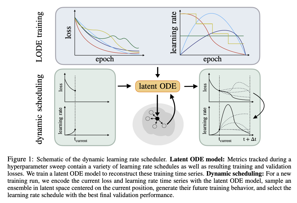
This is like giving our robot optimizer (henceforth roboptimizer) a map of the predicted terrain ahead which has been compiled by previous mechanical explorers journeys (aka training runs). We therefore can make decisions based on maximizing a future reward, i.e taking a large step now may not improve current training accuracy, however it may also be the best/only way to get to the best long term performance. Our learning rate schedule, and hence underlying optimization algorithm, is no longer greedy.
Move fast yet surprisingly don't break things

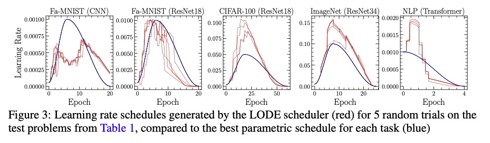
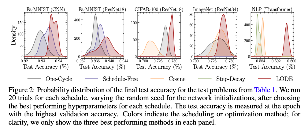
Across Fashion-MNIST, CIFAR-100, ImageNet, and even a Transformer language model, the LODE scheduler performs better than the baselines: cosine, OneCycle, exponential decay, hypergradient descent, schedule-free, and reinforcement learning controllers. Quite surprisingly we see that the best performing learning rate schedules determined by our LODE scheduler often suggests significantly higher learning rates at early times than what we see in the best parametric schedules.
Not only did models reach higher accuracy, they also landed in flatter regions of the loss landscape—which hints towards stronger model generalization.
Key highlights:
- Consistently superior test accuracy across CNNs, ResNets, and Transformers.
- Flatter minima (confirmed via Hessian eigenvalue analysis).
- Computational cost only ~25% higher than simple parametric schedules, but cheaper than RL-based methods.
This insight of very large early step-sizes is not new, and there has been some great work on this phenomena termed the edge of stability, particularly by Jeremy Cohen (who as far as I am aware, coined the term).
Are we truly *learning* the optimisation dynamics?
A natural question here would be how well have we learned a representation of the optimizer dynamics, could we perhaps just always be estimating the same (well performing) schedule for each model/dataset combination?
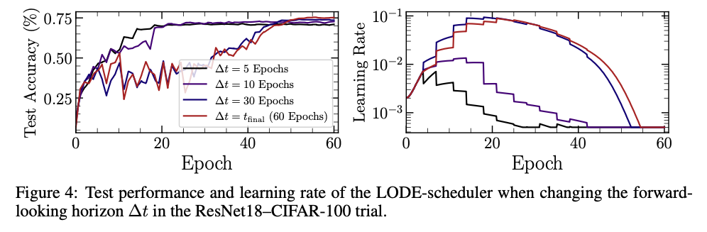
Well, great question, glad you asked. To test this question we may probe the generated schedules and hence training results we get when asking to prioritize results at different times. For example, instead of making a schedule resulting in the best validation loss at the end of training, how about one that minimises this loss after only 50% of the training, what about 10%? The following figure shows the test accuracy, and generated learning rate schedules from the LODE scheduler when asking the validation loss to be minimised at ~8%, 16%, 50%, and 100% of the total training time. We can see if we desire early performance, we can get it with no changes to the scheduler at all (except of course telling it when we want our loss minimized).
While this is clearly not a rigourous proof, it shows at the very least our LODE scheduler understands how to navigate the loss surface to end up in the best minima it can find after an arbitrary amount of exploration time, i.e. we do not always generate the same schedule. This shows that in a way, we can control how greedy we wish our optimizer to be, at least as far as controlling it through the learning rate. Going back to our somewhat contrived analogy, our roboptimizers understand how long they are able to freely explore until they must settle and quickly descend down to the best performing region within their horizon.
Why This Matters
Modern training pipelines already generate tons of metrics during hyperparameter sweeps. The LODE scheduler shows we can recycle that information to learn how to learn. Instead of blindly applying predefined schedules, we can now generate custom, foresight-driven schedules tailored to each task.
This shift could become increasingly important for larger models, where wasted compute and poor convergence are especially costly.
Apart from the practical usefulness of this approach, we also now have a tool that may help improve our understanding of the training dynamics of deep neural networks. It is here that I bring up an intentional ommision so far, we never mentioned the word stochastic. During training, we train all models using some form of stochastic gradient descent or Adam, sometimes with Nesterov momemtum, sometimes without. Now for those of you familiar with latent ODEs, and in fact ODEs in general, you will likely have realised that our LODE scheduler by construction can only generate deterministic trajectories. So what is going on here, how can we learn supposedly stochastic trajectories with a deterministic model? I will not claim to completely understand the answer to this question, and we plan to explore this avenue much more in future work. I will however point out work by the aformention Jeremy Cohen on Central Flows, which aims to understand time averaged dynamics on optimization trajectories in deep learning see here. How stochastic are these gradient descent algorithms really…? (asked in a provocative serif font)
Closing Thoughts
The metaphor of a little robot navigating a treacherous loss surface is helpful to think about here. Previous approaches told the robot that while he is free to choose what direction to walk, he must follow fixed marching orders taking predetermined sized strides, or at best determine the best stride based on his own last few steps. With our latent ODE scheduler, the robot is given a map of the loss surface constructed from past explorations, he is able to anticipate the terrain, and adjusts his stride for the best long-term outcome even if that means suffering a momentary setback.
As models grow in size and complexity, smarter training dynamics like this may be the key to unlocking further breakthroughs in deep learning. There is no use building larger more sophisticated models if we have no reliable way to train them.
Paper: Dynamics of Learning: Generative Schedules from Latent ODEs
Authors: Matt L. Sampson & Peter Melchior
Thank you to GPT-5 for the cute and helpful images, and thank you to the unnamed artists upon which the image generative portion of GPT-5 was trained.
Enjoy Reading This Article?
Here are some more articles you might like to read next: